Introduction A slitless spectrograph is probably the simplest form of spectrograph that an amateur astronomer can build. The three main components of the system are the telescope, diffraction grating, and a detector. Virtually any form of telescope will work as long as it has quality optics and a sturdy mount. The diffraction grating is a transmission grating which is readily available. The detector can be either a photographic or CCD camera. This article explains how to assemble a spectrograph from commercially available components and then calculate the spectral resolution of the instrument. A knowledge of the spectrograph’s resolution is important in astronomical object selection, for example, the spectra of late-type stars (red giants) are typically dominated by wide TiO absorption bands than only require a low resolution spectrograph to study. However, this type of spectrograph would not be suitable for measuring the radial velocity of a nearby star – this would require a much higher resolution. System Overview The spectrograph consists of four commercially available products – a Meade LX200 8" f/6.3 telescope, an SBIG ST-8 CCD camera, a Rainbow Optics transmission grating, and the MIRA 6.0 image processing software. 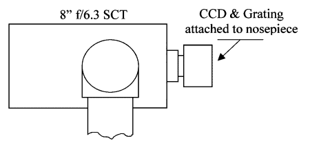
Figure 1 – Diagram of telescope with grating and CCD attached. The term spectrometer refers to any of several types of spectroscopic instruments. A spectrograph is an instrument that records many spectral elements simultaneously with an area detector. The term "slitless" spectrograph can actually refer to two different optical configurations. The first is the spectrograph made by placing the dispersing element, prism or grating, in front of the telescope objective. The second type places the dispersing element between the objective and the focal plane. In this case, the light incident on the prism or grating is a converging beam. This type of spectrograph is also called a "nonobjective" grating spectrograph. Only the second type of "slitless" spectrograph will be discussed in this paper. This type of spectrograph is similar to the Monk-Gillieson spectrograph (Kaneko, et. al.). General spectrometer references are Schroeder (1987) and James. The light ray in figure 2 emerges from the telescope and enters the transmission grating. The grating equation, 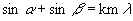 , ,defines the relationship between the entrance angle (  ), deviation angle ( ), deviation angle ( ),
number of grooves per millimeter (m), wavelength ( ),
number of grooves per millimeter (m), wavelength ( ), and the integer number for
the spectrum order (k). In the case of the slitless spectrograph, is 0, and
the grating equation reduces to ), and the integer number for
the spectrum order (k). In the case of the slitless spectrograph, is 0, and
the grating equation reduces to  . .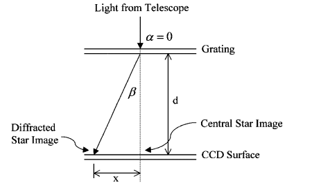
Figure 2 – Diffracted star image produced by a diffraction grating.  . The spectral resolution is a
dimensionless quantity that is a measure of spectral purity (). . The spectral resolution is a
dimensionless quantity that is a measure of spectral purity ().
Spectrographs are considered low resolution when they have R<1000. The plate factor, P, is a measure of the change in wavelength along the surface of the CCD, or  . The plate factor is usually expressed in angstrom per mm. It
can be determined by observing a star’s spectrum that has known features, for
example, the hydrogen lines in an A type star, and using the equation: . The plate factor is usually expressed in angstrom per mm. It
can be determined by observing a star’s spectrum that has known features, for
example, the hydrogen lines in an A type star, and using the equation: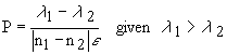 Here, n1 and n2 are the pixel values at  and and  respectively and respectively and  is the linear
size of a pixel. Applying this equation with
n1 = 691.9, n2 =864.4, =6562.8 A, = 4861.3 A, and
= 9x10⁻³ mm yields P = 1094 A/mm. is the linear
size of a pixel. Applying this equation with
n1 = 691.9, n2 =864.4, =6562.8 A, = 4861.3 A, and
= 9x10⁻³ mm yields P = 1094 A/mm.For the case of the Meade LX200 8" f/6.3 telescope, a Rainbow Optics transmission grating, and an SBIG ST-8 CCD, the follow quantities are known:
R = mLk, where L = gratings lit width (portion of grating illuminated by the star’s image from the telescope). 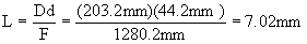 R = (200 g/mm)(7.02 mm)(1) = 1404 at = 6563 A (Hydrogen Alpha line)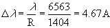 As we shall soon see, the actual resolution of the spectrograph turns out to be much lower. 1. Chromatic Coma The main aberration affecting this system is spectral or chromatic coma. The effect of chromatic coma on the spectral purity is given by (Schroeder 1987)  A characteristic of the coma is that 80% of the energy is concentrated in one half the image spot (Hoag 1970). Taking this into account, the formula for the spectral purity becomes  At = 6563 A and N = 6.3, the spectral purity is = 31 A. As the wavelength
increases so does the chromatic coma. To reduce the effect of the coma on the
spectral purity, a prism can be placed next to the grating, thus forming a "grism".
The design of a grism spectrograph is covered in Bowen, Buil, Gavin, and
Schroeder (1987).2. Field Curvature The aberration due to field curvature results from the cylindrical rather than planar nature of the spectrum’s focus. Referring to figure 2, as the distance x increases from the central star image the focus no longer is directly on the CCD surface. Since astigmatism has only a minor effect on spectral purity, the distance between the sagittal and tangential focal points is assumed to be zero. To quantify the effects of field curvature on resolution, we assume that the focus of the image is a point. Using the property of similar triangles and the geometry in figure 3 the following relationship holds  Combining this with  and solving for and solving for  yields yields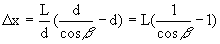 The resolving power becomes  For this spectrograph at = 6563 A,  , L = 7.02mm, and P = 1094 A/mm, the spectral
purity = 67 A. The defocusing effect produced by field curvature significantly
reduces the spectrograph’s resolution. , L = 7.02mm, and P = 1094 A/mm, the spectral
purity = 67 A. The defocusing effect produced by field curvature significantly
reduces the spectrograph’s resolution.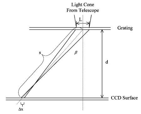
Figure 3 – Field curvature effect geometry In a slitless spectrograph the full width at half maximum (FWHM) of the star’s image becomes the effective entrance slit width for the instrument. The larger the slit width the lower the resolution and spectral resolving power . The spectral
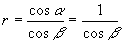
resolving power is given by: , ,where r is the anamorphic factor,
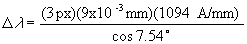
The spectral resolving power becomes 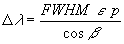 At a wavelength of 6563 A, = 7.54 degrees, and assuming a FWHM of 3 pixels, becomes
For this combination of telescope and camera, each pixel represents 1.45 arc seconds. 4. Sampling Theorem When a continuous signal is sampled, such as a spectra, this process places a lower limit on the spectra purity. Simply put, the sampling theorem states that the highest frequency present in a sampled waveform is one half the sampling rate. The implication of this theorem on the spectrograph is that the smallest value of spectral purity possible is twice the wavelength interval covered by a pixel, or  = (2)(9x10⁻³)(1094 A/mm) = 19.7 A = (2)(9x10⁻³)(1094 A/mm) = 19.7 AFocusing Procedure to Minimize Field Curvature Effect The field curvature aberration essentially produces a defocusing effect on the spectra. To partially correct the problem a simple focusing procedure can be used to minimize the effect. Figure 4 is a 0.5 second exposure of Sirius with the Hydrogen alpha (6563 A), Hydrogen beta (4861 A), and the Fraunhofer A atmospheric water absorption band (band-head at 7594 A) identified. Note that the throughs in the spectrum at approximately column numbers 450 and 620 are artifacts of the CCD spectral response. The Hydrogen beta line will be used to quantify the focus of the telescope/grating system. This procedure will require that the telescope have a focusing aid to obtain the best possible focus of the central star image and a digital readout on the focusing knob. The procedure is as follows:
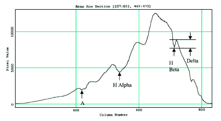
Figure 4 – Spectrum of Sirius focused on central star image 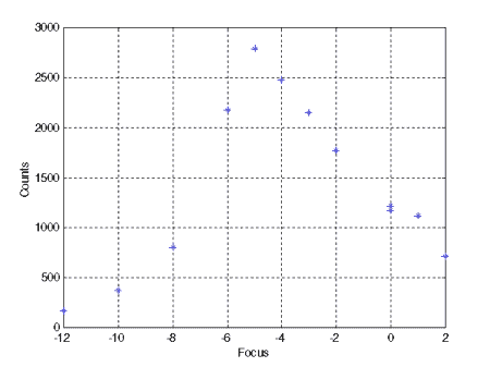
Figure 5 – Variation in the depth of the Hydrogen beta line as the focus is changed. Figure 6 illustrates the effects of focusing has on the Hydrogen lines. Note that the hydrogen lines are deeper and more distinct in figure 6 as compared to the case where the spectrograph is focused on the central star as in figure 4. 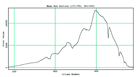
Figure 6 – Spectrum of Sirius focused on the H beta line The resulting spectral purity due to the aberrations of chromatic coma, star’s FWHM, and field curvature are plotted in figure 7. The limitation placed on the spectral purity resulting from the Sampling Theorem where small compared to the aberrations and was not plotted. As illustrated in figure 7, spectral purity is limited by the star’s FWHM to approximately 30 angstrom until 6300 angstroms. After this point the chromatic coma aberration dominates the spectral purity. The focusing procedure previously discussed was employed to reduce the effects of the curvature of field. Note that the curvature of field line in figure 7, labeled "Field", has a minimum at the wavelength of the Hydrogen beta line. Using the spectral purity and wavelength values from figure 7, the resolution varies from R = 138 at 4000 angstroms to R = 213 at 10,000 angstrom. Resolution within this range qualifies this spectrograph as low-resolution. 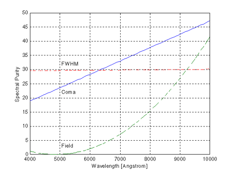
Figure 7 – Spectral purity as a function of wavelength with the effects of each aberration shown separately. [2] Christian Buil’s web site - www.astrosurf.org/buil. [3] Maurice Gavin’s web site - www.astroman.fsnet.co.uk. [4] L.S. Bowen and A.H. Vaughan, Jr., "Nonobjective Gratings", Publications Astronomical Society of the Pacific, vol 85, April 1973, pages 174-176. [5] J.F. James and R.S. Sternberg, "The Design of Optical Spectrometers", Chapman and Hall Ltd., 1969. [6] T. Kaneko, T. Namioka, and M. Seya, "Monk-Gillieson Monochromator", Applied Optics, vol. 10, no. 2, Feb 1971, pages 367-381. [7] A. Hoag and D. Schroeder, "Nonobjective Grating spectroscopy", Publ. Astron. Soc. Pac. 82, pages 1141-1145, 1970. - Ed. BDM |